comexr

Easy acess to Brazilian foreign trade statistics using Apache Arrow.

Eduardo Leoni

2024-07-21

The goal of comexr is to make it easy to download, process, and analyze Brazilian foreign trade statistics, available through the web app http://comexstat.mdic.gov.br/, using the underlying bulk data https://www.gov.br/produtividade-e-comercio-exterior/pt-br/assuntos/comercio-exterior/estatisticas/base-de-dados-bruta.

Installation

##devtools::install_github("leoniedu/comexr")

If you have problems installing arrow, see:

https://arrow.apache.org/docs/r/articles/install.html

Examples

library(comexr)
library(dplyr)
#> 
#> Attaching package: 'dplyr'
#> The following objects are masked from 'package:stats':
#> 
#>     filter, lag
#> The following objects are masked from 'package:base':
#> 
#>     intersect, setdiff, setequal, union

##downloading
#comex_download(years = 2022:2024, types = "ncm", ssl_verifypeer=FALSE)
if (params$download) {
  try(comex_download(years = 2014:2024, types = "ncm"
                     , ssl_verifypeer=FALSE
  ))
}

comex_ncm_f <- comex_ncm()|>filter(year>=2014, year<=2023)

Automatic downloading can be tricky, due to timeout, (lack of) valid security certificates on the Brazilian government websites, along other issues. The code uses the multi_download function from the curl library, so it resumes download if it fails.

Main trade partners, treating countries in Mercosul and European Union as blocks.

Using a programming language like R makes it easy to generate statistics and reports at the intended level of analysis.

msul <- comex("pais_bloco")|>
  filter(block_code==111)|>
  pull(country_code)
#> Rows: 322 Columns: 5
#> ── Column specification ────────────────────────────────────────────────────────
#> Delimiter: ";"
#> chr (4): CO_PAIS, NO_BLOCO, NO_BLOCO_ING, NO_BLOCO_ESP
#> dbl (1): CO_BLOCO
#> 
#> ℹ Use `spec()` to retrieve the full column specification for this data.
#> ℹ Specify the column types or set `show_col_types = FALSE` to quiet this message.
eu <- comex("pais_bloco")|>
  filter(block_code==22)|>
  pull(country_code)
#> Rows: 322 Columns: 5
#> ── Column specification ────────────────────────────────────────────────────────
#> Delimiter: ";"
#> chr (4): CO_PAIS, NO_BLOCO, NO_BLOCO_ING, NO_BLOCO_ESP
#> dbl (1): CO_BLOCO
#> 
#> ℹ Use `spec()` to retrieve the full column specification for this data.
#> ℹ Specify the column types or set `show_col_types = FALSE` to quiet this message.

pb <- comex("pais")|>
  transmute(country_code, 
            partner=
              case_when(country_code%in%msul ~ "Mercosul",
                        country_code%in%eu ~ "European Union",
                        TRUE ~ country_name)
              )
#> Rows: 281 Columns: 6
#> ── Column specification ────────────────────────────────────────────────────────
#> Delimiter: ";"
#> chr (6): CO_PAIS, CO_PAIS_ISON3, CO_PAIS_ISOA3, NO_PAIS, NO_PAIS_ING, NO_PAI...
#> 
#> ℹ Use `spec()` to retrieve the full column specification for this data.
#> ℹ Specify the column types or set `show_col_types = FALSE` to quiet this message.

cstat_top_0 <- comex_ncm_f|>
  left_join(pb) |> 
  group_by(partner)|>
  summarise(fob_usd=sum(fob_usd))|>
  ungroup() |> 
  arrange(desc(fob_usd))|>
  collect()|>
  slice(1:5)

cstat_top <- comex_ncm_f |>
  left_join(pb) |> 
  semi_join(cstat_top_0, by=c("partner"))|>
  group_by(year, partner, direction)|>
  summarise(fob_usd=sum(fob_usd))|>
  collect()

library(ggplot2)
ggplot(aes(x=year, 
           y=fob_usd_bi), 
       data=cstat_top|>
         mutate(fob_usd_bi=fob_usd/1e9)) +
  geom_line(aes(color=partner)) +
  facet_wrap(~direction) +
  labs(color="", x="", y="US$ Bi (FOB)") +
  theme_linedraw() + theme(legend.position="bottom")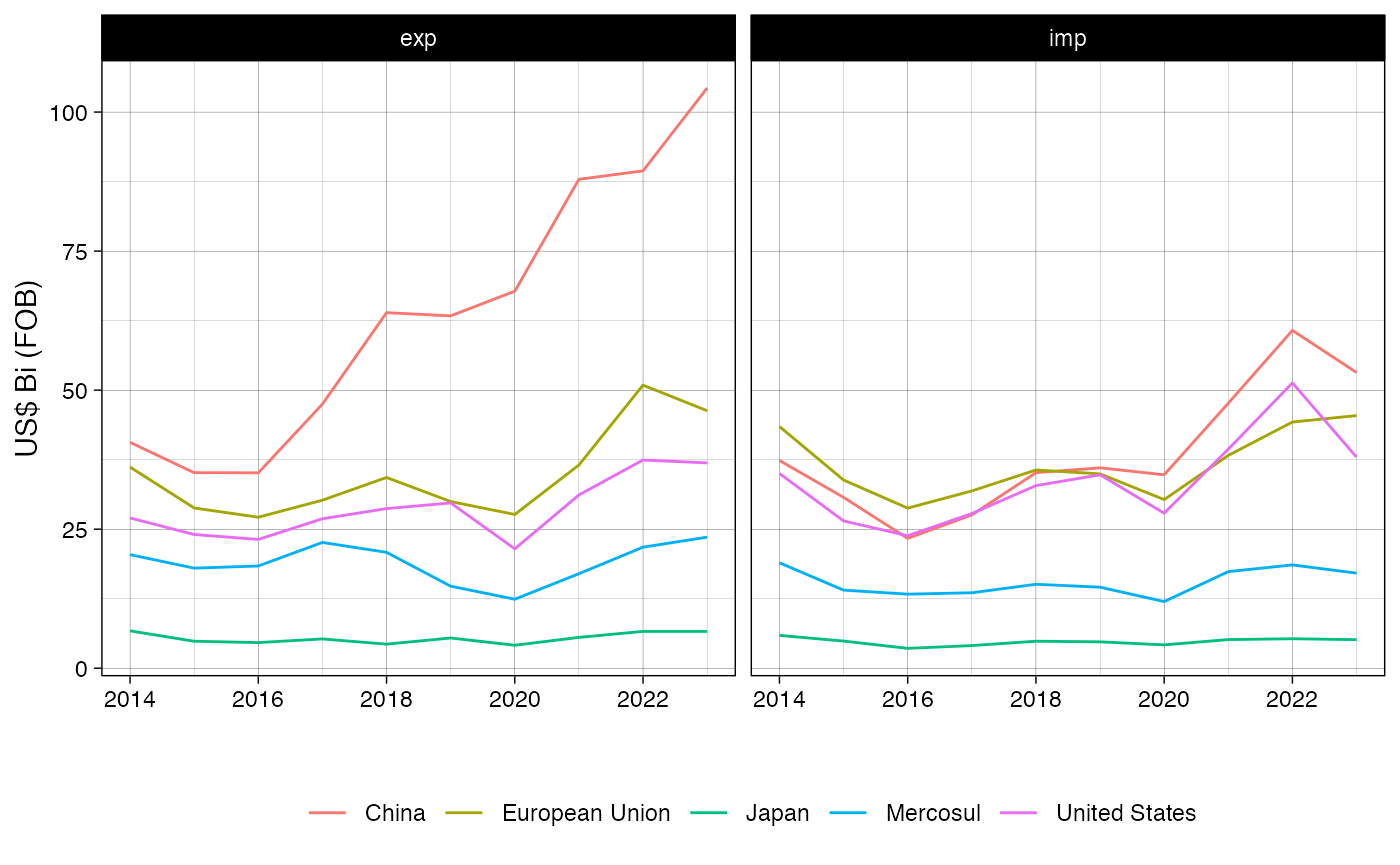

Imports and exports by Brazilian state

You will have access to information not available via the web interface http://comexstat.mdic.gov.br/en/home, such as

bystate <- comex_ncm_f |> 
  group_by(state_abb, year, direction)|>
  summarise(fob_usd=sum(fob_usd))|>
  collect()

topstate <- bystate|>
  group_by(state_abb)|>
  summarise(fob_usd=sum(fob_usd))|>
  arrange(-fob_usd)|>
  head(3)


ggplot(aes(x=year, y=fob_usd_bi, color=state_abb), 
       data=bystate|>
        semi_join(topstate, by="state_abb")|>
        mutate(fob_usd_bi=fob_usd/1e9)) +
  geom_line() +
  facet_wrap(~direction) +
  labs(color="", x="", y="US$ Bi (FOB)") +
  theme_linedraw() + theme(legend.position="bottom")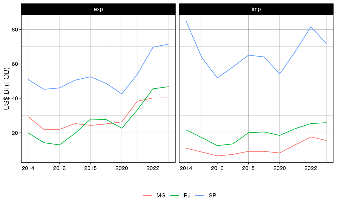

Deflate using CPI (for USD) or IPCA (for BRL) (Experimental)

selected_deflated <- comex_ncm_f%>%
  filter(country_code%in%c(249, 160, 63))%>%
  group_by(direction, date, country_code)%>%
  comex_sum()|>
  comex_deflate()%>%
  collect()

selected_deflated_r <- selected_deflated%>%
  left_join(comex("pais"))%>%
  group_by(direction, country_name)%>%
  arrange(date)%>%
  filter(!is.na(fob_usd))%>%
  comex_roll(x = c("fob_usd_deflated"))
#> Rows: 281 Columns: 6
#> ── Column specification ────────────────────────────────────────────────────────
#> Delimiter: ";"
#> chr (6): CO_PAIS, CO_PAIS_ISON3, CO_PAIS_ISOA3, NO_PAIS, NO_PAIS_ING, NO_PAI...
#> 
#> ℹ Use `spec()` to retrieve the full column specification for this data.
#> ℹ Specify the column types or set `show_col_types = FALSE` to quiet this message.
#> Joining with `by = join_by(country_code)`
  
ggplot(aes(x=date, y=fob_usd_deflated_12/1e9, color=country_name), 
       data=selected_deflated_r)+
  facet_wrap(~direction)+
  geom_line() +
  labs(color="", x="", y="US$ Bi (FOB) Deflated by CPI "%>%paste0(format(max(selected_deflated_r$date), "%m/%Y")), caption = "* 12 month rolling sums") +
  theme_linedraw() + theme(legend.position="bottom") #+ scale_color_manual(values=c("red",  "blue")) 
#> Warning: Removed 33 rows containing missing values or values outside the scale range
#> (`geom_line()`).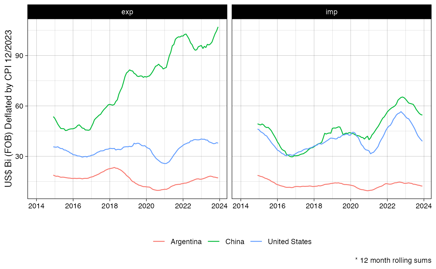

Trade balance

balance_deflated <- comex_ncm_f%>%
  group_by(direction, date)%>%
  comex_sum()%>%
  comex_deflate()%>%
  comex_roll(x = c("fob_brl", "fob_usd", "fob_usd_deflated", "fob_brl_deflated", "cif_usd_deflated", "cif_brl_deflated"))%>%
  collect()

# volume_deflated_r <- balance_deflated%>%
#   group_by(date)%>%
#   summarise(across(matches("^(fob|cif|qt)"), sum))

ggplot(aes(x=date, y=fob_usd_deflated_12/1e9, color=direction), 
       data=balance_deflated) +
  scale_color_manual(values=c("blue", "red")) +
  geom_line() +
  labs(color="", x="", y="US$ Bi (FOB) Deflated by CPI "%>%paste0(format(max(selected_deflated_r$date), "%m/%Y")), caption = "* 12 month rolling sums") +
  theme_linedraw() + 
  geom_vline(xintercept=as.Date("2023-01-01"))+
  theme(legend.position="bottom") #+ scale_color_manual(values=c("red",  "blue")) 
#> Warning: Removed 22 rows containing missing values or values outside the scale range
#> (`geom_line()`).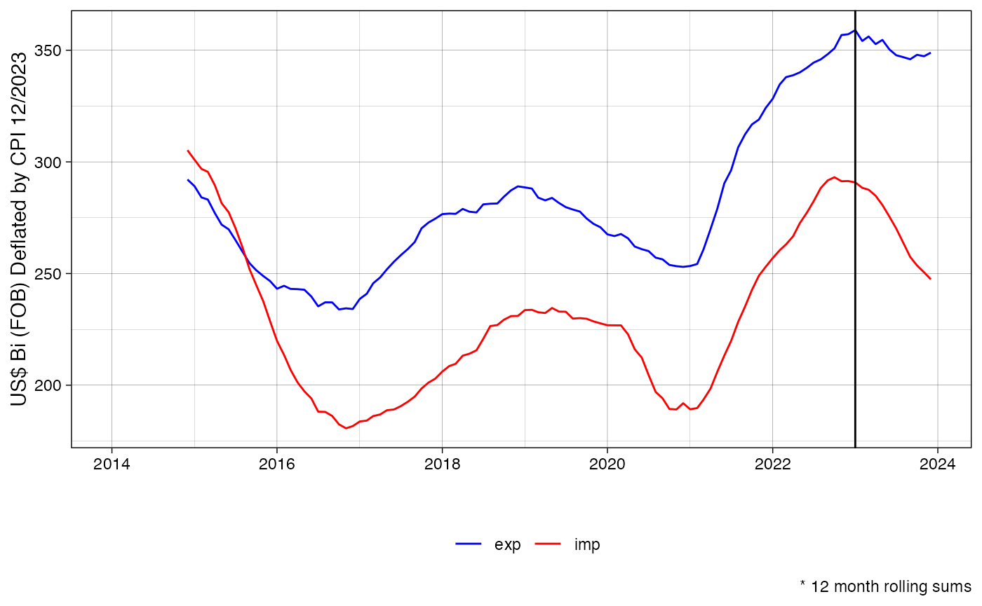

usdmax <- balance_deflated%>%
  group_by(direction)%>%
  arrange(desc(fob_usd_deflated/1e9))%>%
  slice(1)

ggplot(aes(x=date, y=fob_usd_deflated_12/1e9, color=direction), 
       data=balance_deflated) +
  geom_line(aes(y=fob_usd_12/1e9), linetype=2) +
  scale_color_manual(values=c("blue", "red")) +
  geom_line() +
  #geom_line(aes(y=vl_fob_usd_bi), linetype='dashed')+
  labs(color="", x="", y="USD Bi (FOB) Deflated by CPI "%>%paste0(format(max(selected_deflated_r$date), "%m/%Y")), caption = "* 12 month rolling sums", title="Deflated by CPI vs Nominal",
       subtitle = glue::glue("Max of 12 month exports value occurred on {usdmax%>%filter(direction=='exp')%>%pull(date)},\n imports on {usdmax%>%filter(direction=='imp')%>%pull(date)}")) +
  theme_linedraw() + 
  geom_vline(xintercept=as.Date("2023-01-01"))+
  theme(legend.position="bottom") #+ scale_color_manual(values=c("red",  "blue")) 
#> Warning: Removed 22 rows containing missing values or values outside the scale range
#> (`geom_line()`).
#> Removed 22 rows containing missing values or values outside the scale range
#> (`geom_line()`).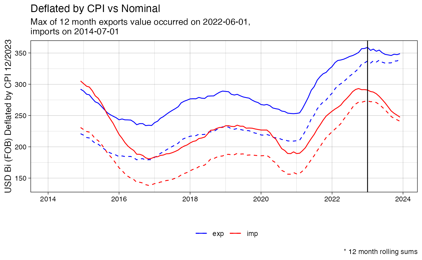

brlmax <- balance_deflated%>%
  group_by(direction)%>%
  arrange(desc(fob_brl_deflated/1e9))%>%
  slice(1)

ggplot(aes(x=date, y=fob_brl_deflated_12/1e9, color=direction), 
       data=balance_deflated) +
  scale_color_manual(values=c("blue", "red")) +
  geom_line() +
  #geom_line(aes(y=vl_fob_usd_bi), linetype='dashed')+
  labs(color="", x="", y="R$ Bi (FOB) Deflated by IPCA "%>%paste0(format(max(selected_deflated_r$date), "%m/%Y")), caption = "* 12 month rolling sums", title="Deflated by IPCA",
       subtitle = glue::glue("Max of 12 month exports value occurred on {brlmax%>%filter(direction=='exp')%>%pull(date)},\n imports on {brlmax%>%filter(direction=='imp')%>%pull(date)}")) +
  theme_linedraw() + 
  geom_vline(xintercept=as.Date("2023-01-01"))+
  theme(legend.position="bottom") #+ scale_color_manual(values=c("red",  "blue")) 
#> Warning: Removed 22 rows containing missing values or values outside the scale range
#> (`geom_line()`).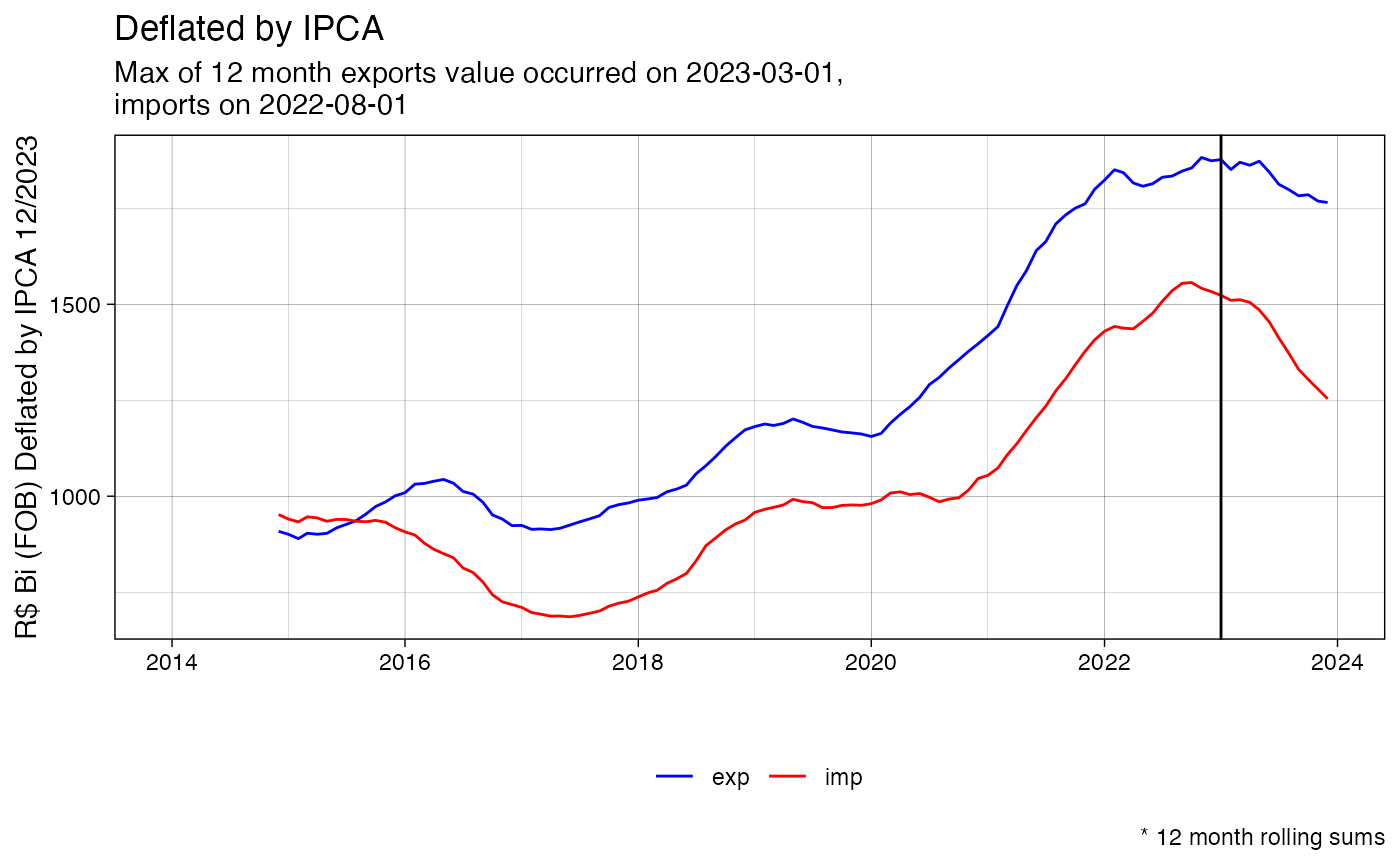

Last month

ggplot(aes(x=date, y=fob_brl_deflated_12/1e9, color=direction), 
       data=balance_deflated%>%filter(lubridate::month(date)==lubridate::month(max(balance_deflated$date)))
       ) +
  scale_color_manual(values=c("blue", "red")) +
  geom_line() +
  geom_line(aes(y=fob_brl_12/1e9), linetype='dashed') +
  #geom_point(aes(y=fob_brl_bi), linetype='dashed') +
  labs(color="", x="", y="R$ Bi (FOB) Deflated by IPCA "%>%paste0(format(max(selected_deflated_r$date), "%m/%Y")), caption = "* 12 month rolling sums") +
  theme_linedraw() + 
  geom_vline(xintercept=as.Date("2024-01-01"))+
  theme(legend.position="bottom") #+ scale_color_manual(values=c("red",  "blue"))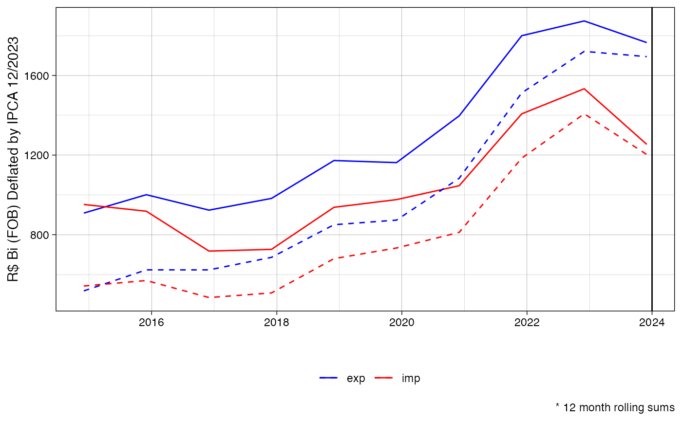 

ggplot(aes(x=date, y=balance_usd_deflated_12), 
       data=
         balance_deflated%>%
         group_by(date)%>%
         arrange(desc(direction))%>%
         summarise(balance_usd_deflated_12=fob_usd_deflated_12[2]/1e9-fob_usd_deflated_12[1]/1e9))+
  #scale_color_manual(values=c("blue", "red")) +
  geom_line()  +
  labs(color="", x="", y="USD$ Bi (FOB) Deflated by CPI "%>%paste0(format(max(selected_deflated_r$date), "%m/%Y")), caption = "* 12 month rolling sums") +
  theme_linedraw() + 
  theme(legend.position="bottom") #+ scale_color_manual(values=c("red",  "blue")) 
#> Warning: Removed 11 rows containing missing values or values outside the scale range
#> (`geom_line()`).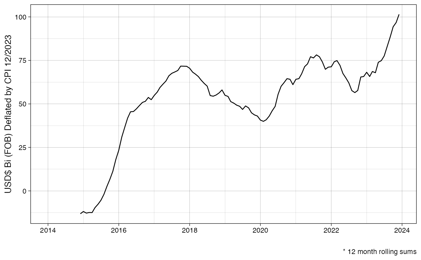

BRL

ggplot(aes(x=date, y=balance_brl_deflated_12), 
       data=
         balance_deflated%>%
         group_by(date)%>%
         arrange(desc(direction))%>%
         summarise(balance_brl_deflated_12=fob_brl_deflated_12[2]/1e9-fob_brl_deflated_12[1]/1e9)%>%
         na.omit()
                   )+
  #scale_color_manual(values=c("blue", "red")) +
  geom_line()  +
  labs(color="", x="", y="R$ Bi (FOB) Deflated by CPI "%>%paste0(format(max(selected_deflated_r$date), "%m/%Y")), caption = "* 12 month rolling sums") +
  theme_linedraw() + 
  theme(legend.position="bottom") #+ scale_color_manual(values=c("red",  "blue"))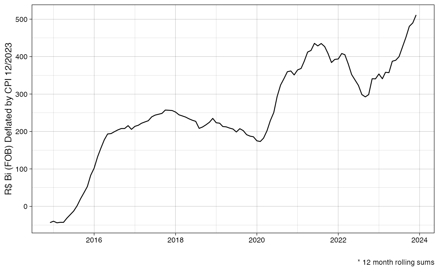 

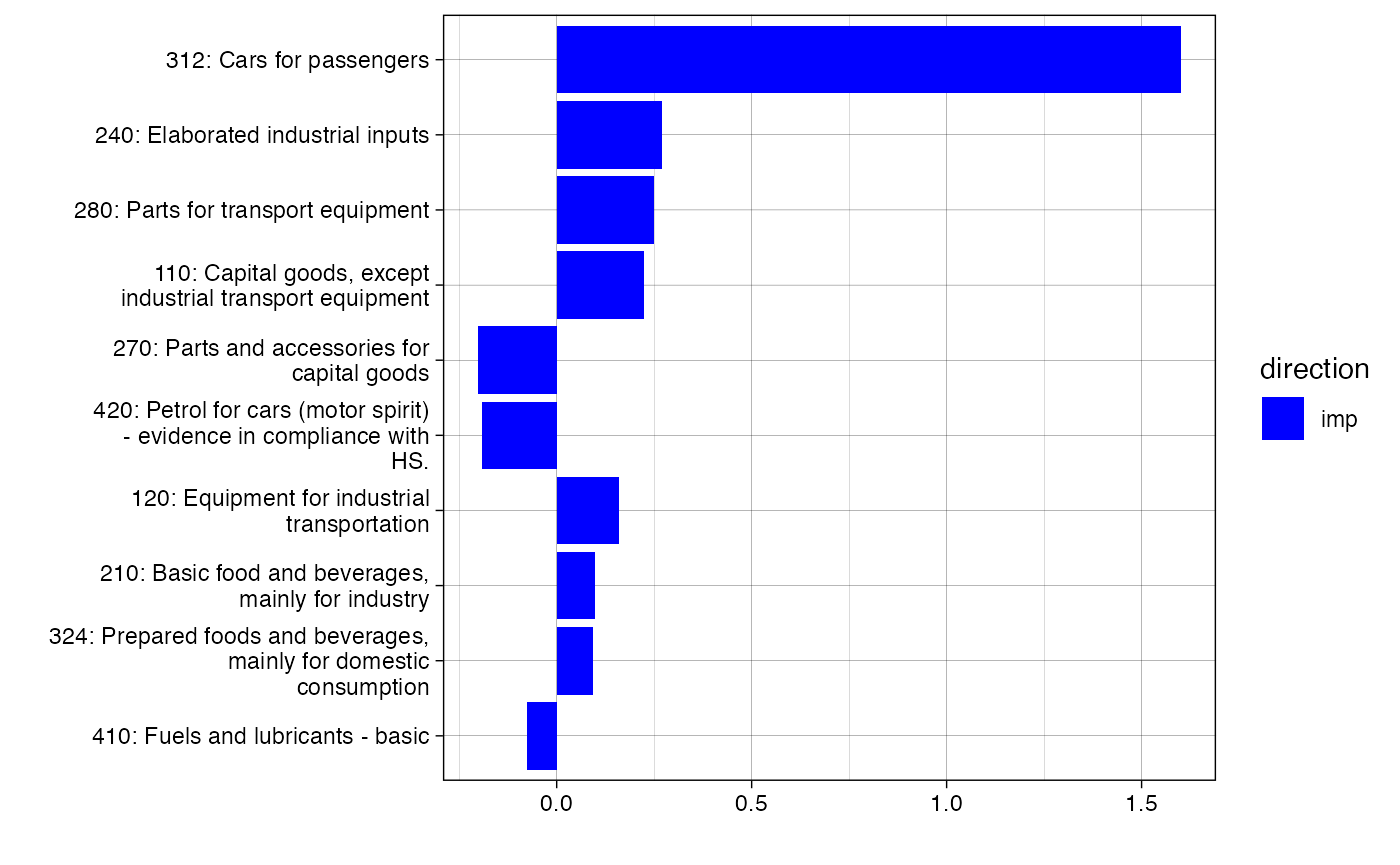
By CGCE

by_cat_0 <- comex_ncm() |> 
  filter(date>="2022-01-01")%>%
  filter(## usa
         #country_code==249
         ## china
         #country_code==160
         ) |>
  left_join(ncms()%>%select(ncm=co_ncm, 
                            name=no_cgce_n3_ing, code=co_cgce_n3
                            #name=no_ncm_ing, code=co_ncm
                            ))|>
  group_by(name,code, direction, date)|>
  comex_sum()|>
  comex_deflate()%>%
  filter(!is.na(fob_brl_deflated))

by_cat_1 <- by_cat_0%>%
  filter(direction=="imp")%>%
  group_by(name,code, direction)|>
  comex_roll(k=1)%>%
  rename_with(function(x) gsub("_1$", "_k", x))%>%
  ungroup%>%
  filter(lubridate::month(date)==lubridate::month(max(date)))%>%
  mutate(year=lubridate::year(date))%>%
  filter(year>=(max(year)-1))%>%
  mutate(year=factor(year,labels = c("last", "current")))

by_cat_2 <- by_cat_1%>%
  select(name,code, direction, fob_usd_deflated_k, year)%>%
  tidyr::pivot_wider(names_from=c("year"), values_from = fob_usd_deflated_k)%>%
  mutate(current=tidyr::replace_na(current, 0),
         last=tidyr::replace_na(last, 0),
    d=current-last, s=last+current, p=current/last)

by_cat <- by_cat_2%>%
  group_by(code)%>%
  summarise(total=sum(abs(current-last)))%>%
  arrange(desc(total))%>%
  head(10)%>%
  inner_join(by_cat_2)%>%
  arrange(total)
#> Joining with `by = join_by(code)`

ggplot(aes(y=label, x=d/1e9, fill=direction), data=by_cat%>%mutate(label=forcats::fct_inorder(paste0(code, ": ", stringr::str_wrap(name,30))))) + geom_col(position="dodge")+ labs(x="", y="") +
  scale_fill_manual(values=c("blue", "red")) +
  theme_linedraw()